1. Trust Region Policy Optimization (TRPO)

TRPO improves a policy monotonically by maximizing a surrogate advantage inside a trust region measured with KL divergence. Use it when policy-gradient updates must stay stable, and as the reference that later methods such as PPO simplify.

Reading time

13 min

Length

2,371 words

Updated

Sep 15, 2026

Total views

--

#math/random-state-functions#math/total-variation-divergence#reinforcement-learning/TRPO

1. Introductions & Preliminaries

What is so-called reinforced learning
The reinforced learning is a computational approaches by emphasizing on the learning by an agent from direct interaction with its environment

(1) Concepts of TRPO

1. Concepts of random state functions

The trust region policy optimization (TRPO)^[1] is a gradient-based method optimization algorithm, the variants of TRPO includes the vine method and the single-path method.

• single-path method can be applied in the model-free-settings
• vine method requires the system to be restored to particular states.

1. Firstly, we define the following Markov decision process^[2] :

$$\begin{array}{}\text{(1.1.1)}& (\mathcal{S},\mathcal{A},P,r,{\rho }_0,\gamma )\end{array}$$

We note except the concepts in original statement, the ${\rho }_0$ : $\mathcal{S}\to \mathbb{R}$ is the distribution of the initial state $s_0$, then $\gamma \in (0,1)$ is discount factor.

The reinforced learning process is a kind of

2. Random state functions

Firstly, we define the following 3 random state functions for optimization :

Random state functions

1. Definition of state-action-value function $Q_{\pi }$, defined as the average reward on all available current state and action :

$$\begin{array}{}\text{(state-action-value-function)}& Q_{\pi }(s_t,a_t)={\mathbb{E}}_{s_{t+1},a_{t+1},\dots }[\sum _{l=0}^{\mathrm{\infty }}{\gamma }^{l}r(s_{t+l})]\end{array}$$

$Q_{\pi }$ fixes both the state $s_t$​ and the action $a_t$, representing the result when take specific action $a_t$. And $l$ is the foresight. This describes the recent reward when we take action $a_t$ at time $t$.

2. The no-policy value function $V_{\pi }$ , we note here the input action of this step $a_t$ is not defined, so :

$$\begin{array}{}\text{(value-function)}& V_{\pi }(s_t)={\mathbb{E}}_{a_t,s_{t+1},\dots }[\sum _{l=0}^{\mathrm{\infty }}{\gamma }^{l}r(s_{t+l})]\end{array}$$

In this function, the action $a_t$ is not given, drawn from the policy $a_t\sim \pi (\cdot |s_t)$

3. The advantage function $A_{\pi }$ is :

$$\begin{array}{}\text{(advantage-function)}& A_{\pi }(s,a)=Q_{\pi }(s,a)-V_{\pi }(s)\end{array}$$

where the $a_t\sim \pi (a_t|s_t)$ is current-step action, and $s_{t+1}\sim P(s_{t+1}|s_t,a_t)$ is the next state, and this is affected by the current state $s_t$ and action $a_t$, for every $t\ge 0$

We note in above theorem, the $A_{\pi }$ gives the advantage of the specific action on specific state

Also note the definition of the above random-state function in ^[3] is different, which is :

$$\begin{array}{}\text{(1.1.2)}& V_{\pi }(s)\equiv (1-\gamma )\mathbb{E}[\sum _{l=0}^{\mathrm{\infty }}{\gamma }^{l}r(s_{t+l})]\end{array}$$

state-action value :

$$\begin{array}{}\text{(1.1.3)}& Q_{\pi }(s,a)\equiv (1-\gamma )R(s,a)+\gamma \mathbb{E}[V_{\pi }(s^{\prime })]\end{array}$$

The difference is that the (1.1.2~3) is normalized by following factor :

$$\begin{array}{}\text{(1.1.4)}& \sum _{t=0}^{\mathrm{\infty }}{\gamma }^l=\frac{1}{1-\gamma }\end{array}$$

3. Average Notations under specific policy

For a policy with

$$\begin{array}{}\text{(1.1.5)}& {\mathbb{E}}_{\tau \sim \tilde{\pi }}\left[X\right]=\sum _{\tau }{P}_{\tilde{\pi }}(\tau )[X]\end{array}$$

where $P_{\tilde{\pi }}$ is the model decision under specific state and actions, defined by (2.1.2)^[2:1]. Since the action is defined on the current state of policy, This can be further expand as (we note $s$ is kept ):

$$\begin{array}{}\text{(1.1.6)}& {\mathbb{E}}_{\tau \sim \tilde{\pi }}[X]=\frac{1}{N}\sum _{i=1}^N{P}_{\tilde{\pi }}(\tau )X(\tau )\end{array}$$

In the second term in equation , the $s$ is the same

We note we also use following notation :

$$\begin{array}{}\text{(1.1.7)}& {\mathbb{E}}_{s\sim d_{\tilde{\pi }},a\sim \tilde{\pi }(\cdot |s)}\end{array}$$

(2) Expected discounted reward

Here the $\pi$ is a policy that determines the result state. denoted by $\pi :\mathcal{S}\times \mathcal{A}\to [0,1]$, the $\eta (\pi )$ denotes the expected discounted reward, as given in (2.4.1)^[2:2], (2.3.3)^[2:3]. which can be rewritten as The sum of the as-far reward:

$$\begin{array}{}\text{(1.2.1)}& \boxed{{\displaystyle \eta (\pi )={\mathbb{E}}_{s_0,a_0,\dots }[\sum _{t=0}^{\mathrm{\infty }}{\gamma }^{t}r(s_t)]}}\end{array}$$

The initial state is given by:

$$\begin{array}{}\text{(1.2.2)}& s_0\sim {\rho }_0(s_0),a_t\sim \pi (a_t|s_t),s_{t+1}\sim P(s_{t+1}|s_t,a_t)\end{array}$$

(3) Policy Relation Theorem

Then, the expected return of another policy $\tilde{\pi }$ in the terms of advantage over $\pi$ can be given as follows, compare to (1.2.1), we should state following lemma :

Policy relation

$$\begin{array}{}\text{(policy-relation)}& \boxed{{\displaystyle \eta (\tilde{\pi })=\eta (\pi )+{\mathbb{E}}_{\tau \sim \tilde{\pi }}[\sum _{t=0}^{\mathrm{\infty }}{\gamma }^t{A}_{\pi }(s_t,a_t)]}}\end{array}$$

Such expectation is taken over the trajectory $\tau :=(s_0,a_0,s_1,a_1,\dots )$

To derive Lemma. region-policy-relation,.We know from (3.1.1)^[2:4] that, for a fixed policy $\pi$, we have :

$$\begin{array}{}\text{(1.3.1)}& V_{\pi }(s)={\mathbb{E}}_{a\sim \pi (\cdot |s)}[r(s,a)+\gamma V_{\pi }(s)]\end{array}$$

Then $Q$ is, since $a$ is already determined, we have :

$$\begin{array}{}\text{(1.3.2)}& Q_{\pi }(s,a)={\mathbb{E}}_{\pi }[r(s)+\gamma V_{\pi }(s)]\end{array}$$

We also note here that the optimal policy gives :

$$\begin{array}{}\text{(1.3.3)}& V^{\ast }(s)=\underset{a}{max}{Q}^{\ast }(s,a)\end{array}$$

Substituting (1.3.2) into (advantage-function), we use the $Q$ as the real value function :

$$\begin{array}{}\text{(1.3.4)}& A_{\pi }(s,a)={\mathbb{E}}_{\pi }[r(s)+\gamma V_{\pi }(s^{\prime })-V_{\pi }(s)]\end{array}$$

For a specific time $t$, the $\mathbb{E}$ automatically disappear, then :

$$\begin{array}{}\text{(1.3.5)}& A_{\pi }(s_t,a_t)=r(s_t)+\gamma V_{\pi }(s_{t+1})-V_{\pi }(s_t)\end{array}$$

Then, we prove from (policy-relation), here :

$$\begin{array}{}\text{(1.3.6)}& {\mathbb{E}}_{\tau \sim \tilde{\pi }}\left[\sum _{t=0}^{\mathrm{\infty }}{\gamma }^t{A}_{\pi }\right]={\mathbb{E}}_{\tau \sim \tilde{\pi }}\left[\sum _{t=0}^{\mathrm{\infty }}({\gamma }^{t+1}{V}_{\pi }(s_{t+1})-{\gamma }^t{V}_{\pi }(s_t)+{\gamma }^{t}r(s_t))\right]={\mathbb{E}}_{r\sim \tilde{\pi }}[\sum _{t=0}^{\mathrm{\infty }}{\gamma }^{t}r(s_t)-V_{\pi }(s_0)]\end{array}$$

So using (1.2.1), we have :

$$\begin{array}{}\text{(1.3.7)}& {\mathbb{E}}_{\tau \sim \tilde{\pi }}\left[\sum _{t=0}^{\mathrm{\infty }}{\gamma }^t{A}_{\pi }\right]=\eta (\tilde{\pi })-{\mathbb{E}}_{s_0\sim {\rho }_0}[V_{\pi }(s_0)]\end{array}$$

Since starting from $s_0\sim {\rho }_0$, Using (value-function), also using (1.2.1), since $t=0$ we have :

$$\begin{array}{}\text{(1.3.8)}& V_{\pi }(s_0)=\sum _{l=0}^{\mathrm{\infty }}{\gamma }^{l}r(s_t)\to \mathbb{E}[V_{\pi }(s_0)]=\eta (\pi )\end{array}$$

the expected return under policy is ${\eta }_{\pi }=\mathbb{E}[V_{\pi }(s_0)]$, then (policy-relation) holds, so the proof completes.

(4) Visitation Frequencies

We let the ${\rho }_{\pi }$ be the unnormalized discounted visitation frequencies.

$$\begin{array}{}\text{(1.4.1)}& {\rho }_{\pi }(s)=P(s_0=s)+\gamma P(s_1=s)+{\gamma }^{2}P(s_2=s)+\dots \end{array}$$

This is the sum of the possibility to visit a specific state over some time. This is positive on every term. The ${\rho }_{\pi }$ is called visitation frequency density.

Using the relation (policy-relation), we can expand it using (1.1.5), we also limit the result state and action, i.e., $s_t=s,a_t=a$. on a deterministic states $s$ and the available actions $a$, so the policy is written as $\tilde{\pi }(a|s)$, then we sum all the probability that under that policy, on all the possible states at time $t$.

Since the state on any $s$ at all $t$ under a trajectory, can be summed by $t$, then :

$$\begin{array}{}\text{(1.4.2)}& {\mathbb{E}}_{\tau \sim \tilde{\pi }}[\sum _{t=0}^{\mathrm{\infty }}{\gamma }^t{A}_{\pi }(s,a)]=\sum _s\sum _{t=0}^{\mathrm{\infty }}P(s_t=s|\tilde{\pi })\sum _a\tilde{\pi }(a|s){\gamma }^t{A}_{\pi }(s,a)\end{array}$$

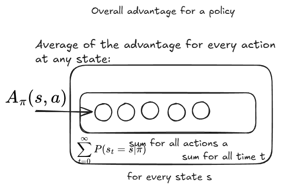
Title To help to understand above equations,
We note that A policy $\tilde{\pi }$ is a rule or probability distribution for selecting actions, which is often a distribution of the next action :

$$\pi (a|s)=\{\begin{array}{l}1\text{if }a\text{ is chosen at some state }s\\ 0\text{ otherwise}\end{array}$$

For example :

$$\tilde{\pi }(a_1|s)=0.7\tilde{\pi }(a_1|s)=0.3$$

then we substitute $\rho$ here, we got :

$$\begin{array}{}\text{(1.4.3)}& \eta (\tilde{\pi })=\eta (\pi )+\sum _s{\rho }_{\tilde{\pi }}(s)\sum _a\tilde{\pi }(a|s)A_{\pi }(s,a)\end{array}$$

For any policy update $\pi \to \tilde{\pi }$ if we ensure that :

$$\begin{array}{}\text{(1.4.4)}& \boxed{{\displaystyle \sum _a\tilde{\pi }(a|s)A_{\pi }(s,a)>0}}\end{array}$$

then the performance of policy $\eta$ is ==guaranteed to increase==. But due to the estimation and approximation error.

(5) Local Approximation of performance

The model training process is a process of optimizing the policy. From (1.4.3), we change the $\tilde{\pi }$ in $\rho$ to the $\pi$, we get the approximation by substituting to visitation frequency ${\rho }_{\pi }$ :

$$\begin{array}{}\text{(1.5.1)}& \boxed{{\displaystyle L_{\pi }(\tilde{\pi })=\eta (\pi )+\sum _s{\rho }_{\pi }(s)\sum _a\tilde{\pi }(a|s)A_{\pi }(s,a)}}\end{array}$$

Subs the $\pi$ into above part, we have :

$$L_{\pi }(\pi )=\eta (\pi )$$

always satisfied

We note if, we have a policy that parametrized by $\theta$, i.e., ${\pi }_{\theta }(a|s)$, which is a differentiable function of the parameter vector $\theta$, then, $L_{\pi }$ matches $\eta$ to first order. We have that for any parameter value set ${\theta }_0$, we should make that :

$$\begin{array}{}\text{(1.5.2)}& L_{{\pi }_{{\theta }_0}}({\pi }_{\theta })=\eta ({\pi }_{{\theta }_0})\end{array}$$

satisfying :

$$\begin{array}{}\text{(1.5.3)}& {\mathrm{\nabla }}_{\theta }{L}_{{\pi }_{{\theta }_0}}({\pi }_{\theta }){|}_{\theta ={\theta }_0}={\mathrm{\nabla }}_{\theta }{\eta }_{{\pi }_{\theta }}{|}_{\theta ={\theta }_0}\end{array}$$

We note that, for a sufficiently small step ${\pi }_{{\theta }_0}\to \pi$, we can use (1.5.2) to substitute $\eta$ in (1.4.3). So the new policy ${\pi }_{new}$ should be defined as following policy update criterion :

$$\begin{array}{}\text{(1.5.4)}& \boxed{{\displaystyle {\pi }_{new}(a|s)=(1-\alpha ){\pi }_{old}(a|s)+\alpha {\pi }^{\prime }(a|s)}}\end{array}$$

In ^[3:1], the lowest bound is derived as :

$$\begin{array}{}\text{(1.5.5)}& \boxed{{\displaystyle \eta ({\pi }_{new})\ge {\eta }_{{\pi }_{old}}({\pi }_{new})-\frac{2ϵ\gamma }{(1-\gamma {)}^2}{\alpha }^2}}\end{array}$$

where :

$$\begin{array}{}\text{(1.5.6)}& ϵ=\underset{s}{max}\left|{\mathbb{E}}_{a\sim {\pi }^{\prime }(a|s)}[A_{\pi }(s,a)]\right|\end{array}$$

note (1.5.5) only applies to mixture policies generated by (1.5.4). This policy class is unwieldly and restrictive in practice.

2. Monotonic Improvement guarantee

(1) Introduction

For the lowest bound by (1.5.5), this is a principle applied into general stochastic policy classes (rather than just mixed classes of (1.5.4)). For all the possible policies, the (1.5.4) is often desired.

The Total Variation divergence is used for the distance measure, defined as half of Manhattan distance :

$$\begin{array}{}\text{(2.1.1)}& D_{TV}(p||q)=\frac{1}{2}\sum _i|p_i-q_i|\end{array}$$

We define we total variation distance $D_{TV}$ between two policies, is :

$$\begin{array}{}\text{(2.1.2)}& D_{TV}^{max}(\pi ,\tilde{\pi })=\underset{s}{max}{D}_{TV}(\pi (\cdot |s)||\tilde{\pi }(\cdot |s))\end{array}$$

In (1.5.4), we have :

Total variation distance theorem
The theorem is that, if we set $\alpha =D_{TV}^{max}({\pi }_{old}||{\pi }_{new})$, we have, the following relation holds :

$$\begin{array}{}\text{(total-variation-distance)}& \{\begin{array}{ll}& \eta ({\pi }_{new})\ge L_{{\pi }_{old}}({\pi }_{new})-\frac{4ϵ\gamma }{(1-\gamma {)}^2}{\alpha }^2\\ \text{where}& ϵ=\underset{s,a}{max}|A_{\pi }(s,a)|\end{array}\end{array}$$

(2) Using KL divergence to express

In (total-variation-distance), the $\alpha$ is held for the $\alpha =D_{TV}^{max}$, we have the relation between the total variation divergence and the KL divergence ^[4], stated as :

$$\begin{array}{}\text{(2.2.1)}& \boxed{{\displaystyle D_{TV}(p||q{)}^2\le D_{KL}(p||q)}}\end{array}$$

Similar to (2.1.2), We still use a max notation to the KL divergence for policy difference (on all states) :

$$\begin{array}{}\text{(2.2.2)}& D_{KL}^{max}(\pi ,\tilde{\pi })=\underset{s}{max}{D}_{KL}(\pi (\cdot |s)||\tilde{\pi }(\cdot |s))\end{array}$$

We also have the relationship between the total variation divergence and the KL divergence, as :

$$\begin{array}{}\text{(2.2.3)}& \boxed{{\displaystyle \eta (\tilde{\pi })\ge L_{\pi }(\tilde{\pi })-\frac{4ϵ\gamma }{(1-\gamma {)}^2}{D}_{KL}^{max}(\mathit{\pi },\tilde{\pi })}}\end{array}$$

in later derivations, we set $C=\frac{4ϵ\gamma }{(1-\gamma {)}^2}$

To maximize $\eta (\tilde{\pi })$ in the next iteration, we got the following optimization steps (here $L$ is defined by (1.5.1)) :

$$\begin{array}{}\text{(2.2.4)}& {\pi }_{i+1}\leftarrow \arg \underset{\pi }{max}\left[\underset{M_i(\pi )}{\underbrace{L_{{\pi }_i}(\pi )-C{D}_{KL}^{max}({\pi }_i,\pi )}}\right]\end{array}$$

Here $M$ is a surrogate function that memorize $\eta$. Thus we have :

$$\begin{array}{}\text{(2.2.5)}& \eta ({\pi }_{i+1})-\eta ({\pi }_i)\ge M_i({\pi }_{i+1})-M_i({\pi }_i)\end{array}$$

The Trusted region policy optimization is an approximation of the algorithm (2.2.4). Such a policy uses constraint on the KL divergence rather than a penalty.

3. Trusted Region Policy Optimization

(1) Parameterized Policy

We considerate the optimization of the parameterized policy, i.e., ${\pi }_{\theta }(a|s)$ with the parameter vector $\theta$, so that, we can express the notations on the policy by $\theta$, e.g. (1.5.1) and (2.2.3) as :

$$\begin{array}{}\text{(3.1.1)}& L(\theta ):=L_{{\pi }_{\theta }}({\pi }_{\theta })\eta (\theta ):=\eta ({\pi }_{\theta })\end{array}$$

The target is to maximize $M(\theta )$, i.e., :

$$\begin{array}{}\text{(3.1.2)}& \boxed{{\displaystyle {\text{maximize}}_{\theta }[L_{{\theta }_{old}}(\theta )-C{D}_{KL}^{max}({\theta }_{old},\theta )]}}\end{array}$$

Trusted region policy constraint
In the practical case, since $D_{KL}$ is always positive, we can make the second term as small as possible, then, the trust region constraint is constructed as :

$$\begin{array}{}\text{(trusted-region-policy)}& \{\begin{array}{l}{\text{maximize}}_{\theta }{L}_{{\theta }_{old}}(\theta )\\ \text{subject to}{D}_{KL}^{max}({\theta }_{old},\theta )\le \delta \end{array}\end{array}$$

Here $\theta (a|s)$ depends on the available actions states.

We note the problem in Theorem. TRPO is a problem solved in the KL divergence bounded space, but such a problem is intractable, (this is because, the $max$ is applied in the firstly equation, so for every state, it impose a new constraint, and in the reinforced learning, there is often a great number of states, and the policy $\theta =\theta (\cdot |s_{1,2,\dots })$ ) depends on the states.

So the second constraint is applied by an average on the states :

$$\begin{array}{}\text{(3.1.3)}& {\bar{D}}_{KL}^{\rho }({\theta }_1,{\theta }_2):={\mathbb{E}}_{s\sim \rho }[D_{KL}({\pi }_{{\theta }_1}(\cdot |s)||{\pi }_{{\theta }_2}(\cdot |s))]\end{array}$$

So (trusted-region-policy) becomes following :

$$\begin{array}{}\text{(3.1.4)}& \boxed{{\displaystyle \{\begin{array}{l}{\text{maximize}}_{\theta }{L}_{{\theta }_{old}}(\theta )\\ \text{subject to}{\bar{D}}_{KL}^{{\rho }_{{\theta }_{old}}}({\theta }_{old},\theta )\le \delta \end{array}}}\end{array}$$

Here $\rho$ is a state distribution used to average the state-wise KL divergence (the states are sampled according to the $\rho$, defined in (1.4.1)).

Usually, the $\rho$ in above equation is chosen as the state visitation distribution under the old policy.

$$\rho ={\rho }_{{\theta }_{old}}$$

i.e., according to the definition,

$$\begin{array}{}\text{(sampling-distribution)}& {\rho }_{\pi }(s)=\sum _{t=0}^{\mathrm{\infty }}{\gamma }^{t}P(s_t=s|\pi )\end{array}$$

Sometimes, the ${\rho }_{\pi }$ is also normalized as following :

$$\begin{array}{}\text{(3.1.5)}& d_{\pi }(s)=(1-\gamma )\sum _{t=0}^{\mathrm{\infty }}{\gamma }^{t}P(s_t=s|\pi )\end{array}$$

4. Sample-based estimation

(1) Problem construction

Since the $L$ is the approximated performance defined in (1.5.1), the optimization problem (3.1.4) is written as :

$$\begin{array}{}\text{(4.1.1)}& \begin{array}{r}\text{maximize}\sum _s{\rho }_{{\theta }_{old}}(s)\sum _a{\pi }_{\theta }{A}_{\pi }(s,a)\\ \text{subject to}{\bar{D}}_{KL}^{{\rho }_{{\theta }_{old}}}({\theta }_{old},\theta )\le \delta \end{array}\end{array}$$

we note under a sampling distribution $q$, the contribution of a single $s_n$ can be expressed by the importance sampling estimator^[5]. That is, we use distribution $a\sim q$ and importance sampling to compute the average :

$$\begin{array}{}\text{(4.1.2)}& \sum _a{\pi }_{\theta }(a|s_n)A_{{\theta }_{old}}(s_n,a)={\mathbb{E}}_{a\sim q(\cdot \mid s_n)}[\frac{{\pi }_{\theta }(a|s_n)}{q(a|s_n)}{A}_{{\theta }_{old}}(s_n,a)]\end{array}$$

then the problem (3.1.4) will become :

$$\begin{array}{}\text{(4.1.3)}& \boxed{{\displaystyle \begin{array}{r}\text{maximize}{\mathbb{E}}_{s\sim {\rho }_{{\theta }_{old}},a\sim q}[\frac{{\pi }_{\theta }(a|s_n)}{q(a|s_n)}{Q}_{{\theta }_{old}}(s_n,a)]\\ \text{subject to}{\mathbb{E}}_{s\sim {\rho }_{{\theta }_{old}}}[D_{KL}({\pi }_{{\theta }_{old}}||{\pi }_{\theta })]\le \delta \end{array}}}\end{array}$$

We note in the (4.1.3), the change from $A$ to $Q$ is valid only as an optimization-equivalence. Considering the (advantage-function),

$$\begin{array}{}\text{(4.1.4)}& {\mathbb{E}}_{a\sim {\pi }_{\theta }}[A_{{\theta }_{\text{old}}}(s,a)]={\mathbb{E}}_{a\sim {\pi }_{\theta }}[Q_{{\theta }_{\text{old}}}(s,a)-\underset{\text{not depend on }\theta }{\underbrace{V_{{\theta }_{\text{old}}}(s)}}]\end{array}$$

in the optimization process, since we want to maximize, the second term in (4.1.4) is a constant and thus can be dropped.

We also note the $s\sim {\rho }_{{\theta }_{old}}$ and $a\sim q$ is the single path sample-based estimation for the objective and constraint.

Another estimation is the Vine method, in which we will choose a subset of $N$ states along these trajectories. We can sample $K$ actions rather than using $a_{n,k}\sim q(\cdot |s_n)$.

In the vine estimation, we can choose any $q(\cdot |s_n)$ with a support that includes the support of ${\pi }_{\theta }(\cdot |s_n)$ will produce a consistent estimator. Using use $q(\cdot |s_n)={\pi }_{{\theta }_i}(\cdot |s_n)$ still works well. This method finally yield following equations. But we will not cover them in detail :

$$L_n(\theta )=\sum _{k=1}^K{\pi }_{\theta }(a_k|s_n)\hat{Q}(s_n,a_k)$$

using the importance sampling like 4.1.2, we also can get :

$$L_n(\theta )=\frac{\sum _{k=1}^K\frac{{\pi }_{\theta }(a_{n,k}|s_n)}{{\pi }_{{\theta }_{old}}(a_{n,k}|s_n)}\hat{Q}(s_n,a_{n,k})}{\sum _{k=1}^K\frac{{\pi }_{\theta }(a_{n,k}|s_n)}{{\pi }_{{\theta }_{old}}}}$$

References

---

1. Schulman, John, Sergey Levine, Philipp Moritz, Michael I. Jordan, and Pieter Abbeel. “Trust Region Policy Optimization.” arXiv:1502.05477. Preprint, arXiv, April 20, 2017. https://doi.org/10.48550/arXiv.1502.05477 ↩︎

2. 1. Markov-decision-process ↩︎ ↩︎ ↩︎ ↩︎ ↩︎

3. Kakade, Sham and Langford, John. Approximately optimal approximate reinforcement learning. In ICML, volume 2, pp. 267–274, 2002. https://people.eecs.berkeley.edu/~pabbeel/cs287-fa09/readings/KakadeLangford-icml2002.pdf ↩︎ ↩︎

4. 2. Kullback-Leibler divergence ↩︎

5. 2. Monte-Carlo Sampling and Importance Sampling ↩︎